Kruschke - ch. 3
Running Proportions
N <- 500
flipseq <- sample(x=c(0,1), size=N, replace=T)
r <- cumsum(flipseq)
runprop <- r/(1:N)
plot(1:N, runprop, type="o", log="x", ylim=c(0,1), col="blue")
abline(h=0.5, lty="dotted")
flipletters <- paste( c("T", "H")[flipseq[1:10] +1], collapse="")
displaystring <- paste("Flip sequence = ", flipletters, "...", sep="")
text(50, 0.8, labels=displaystring)
text(N, 0.2, # coordinates
     paste("End Proportion = ", runprop[N]), # text
     adj=c(1,0) # right aligned
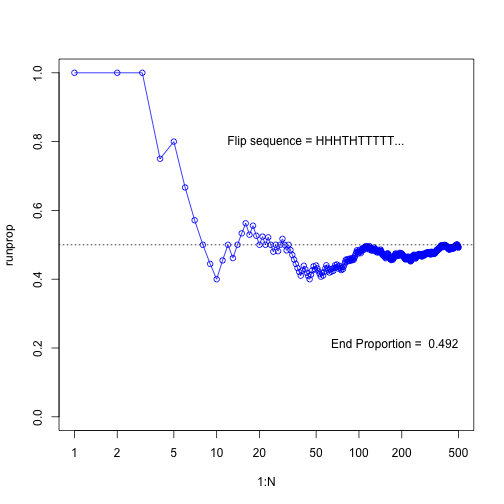
     )
plot of chunk unnamed-chunk-1
dev.copy2pdf(file="/Users/Claudius/Dropbox/Kruschke_Dog_Book/RunningPropportion.pdf")## quartz_off_screen
## 2HairEyeColor
Looking at the data set
show( HairEyeColor ) # built-in data set## Error in eval(expr, envir, enclos): could not find function "show"dim( HairEyeColor ) # a 3-dimensional array## [1] 4 4 2dimnames( HairEyeColor )## $Hair
## [1] "Black" "Brown" "Red" "Blond"
##
## $Eye
## [1] "Brown" "Blue" "Hazel" "Green"
##
## $Sex
## [1] "Male" "Female"class( HairEyeColor ) # an array of integer values## [1] "table"Marginalise over sex and get joint probabilities
# marginalise over the dimension "Sex"
EyeHairFreq = apply( X=HairEyeColor, MARGIN=c("Eye", "Hair"), FUN=sum )
EyeHairFreq
## Hair
## Eye Black Brown Red Blond
## Brown 68 119 26 7
## Blue 20 84 17 94
## Hazel 15 54 14 10
## Green 5 29 14 16class(EyeHairFreq) # 2-dimensional array, aka matrix## [1] "matrix"sum(EyeHairFreq)## [1] 592EyeHairProp = EyeHairFreq / sum(EyeHairFreq)
round(EyeHairProp, 2) # joint probabilities, as in table 4.1## Hair
## Eye Black Brown Red Blond
## Brown 0.11 0.20 0.04 0.01
## Blue 0.03 0.14 0.03 0.16
## Hazel 0.03 0.09 0.02 0.02
## Green 0.01 0.05 0.02 0.03Marginal probabilities of hair and eye color
# get marginal probabilities of Hair color
HairFreq = apply(X=HairEyeColor, MARGIN=c("Hair"), FUN=sum) # the MARGIN argument specifies what dimension to keep
HairProp = HairFreq / sum(HairFreq)
round(HairProp, 2)
## Black Brown Red Blond
## 0.18 0.48 0.12 0.21# get marginal probabilities of Eye color
EyeFreq = apply(X=HairEyeColor, MARGIN=c("Eye"), FUN=sum)
EyeProp = EyeFreq / sum(EyeFreq)
round(EyeProp, 2)## Brown Blue Hazel Green
## 0.37 0.36 0.16 0.11Conditional probability of hair color given blue eye color
round(EyeHairProp, 2)## Hair
## Eye Black Brown Red Blond
## Brown 0.11 0.20 0.04 0.01
## Blue 0.03 0.14 0.03 0.16
## Hazel 0.03 0.09 0.02 0.02
## Green 0.01 0.05 0.02 0.03# joint probs of Blue Eye color and all Hair colors
round(EyeHairProp["Blue",], 2)## Black Brown Red Blond
## 0.03 0.14 0.03 0.16# marginal prob. of blue eye color
EyeProp["Blue"]## Blue
## 0.3631757# conditional prob. of hair colors given eye color is blue
round( EyeHairProp["Blue",] / EyeProp["Blue"], 2)## Black Brown Red Blond
## 0.09 0.39 0.08 0.44\[ p(Hair* | Eye = Blue) = \frac{p(Hair*, Eye = Blue)}{p(Eye = Blue)} \]
Hair* stands for any of the 4 hair colors. The conditional probability of a hair color given blue eye color is the joint probability over the marginal probability of blue eye color, i. e. the proportion of people with blue eyes that also have that specific hair color. With blue eyes the person is clearly much more likely to have blond or brown hair than Black or red. There is clearly a correlation between these two traits, also called linkage disequilibrium.
What is the probability of eye colors given brown hair?
# joint frequencies of eye colors with brown hair
round(EyeHairProp[, "Brown"], 2)
## Brown Blue Hazel Green
## 0.20 0.14 0.09 0.05# marginal probability of brown hair
round(HairProp["Brown"], 2)## Brown
## 0.48# conditional probs of eye colors given brown hair
round(EyeHairProp[, "Brown"] / HairProp["Brown"], 2)## Brown Blue Hazel Green
## 0.42 0.29 0.19 0.10It looks like people with brown hair are much more likely to have brown eyes than green eyes.
Simulate running proportions of flipping a biases coin
N <- 500
pHead = 0.8
flipseq <- sample(x=c(0,1), prob=c(1-pHead, pHead), size=N, replace=T) # Head counts as 1, Tail counts as 0
r <- cumsum(flipseq)
runprop <- r/(1:N)
plot(1:N, runprop, type="o", log="x", ylim=c(0,1), col="blue")
abline(h=0.8, lty="dotted")
flipletters <- paste( c("T", "H")[flipseq[1:10] +1], collapse="")
displaystring <- paste("Flip sequence = ", flipletters, "...", sep="")
text(50, 0.3, labels=displaystring)
text(N, 0.2, # coordinates
     paste("End Proportion = ", runprop[N]), # text
     adj=c(1,0) # right aligned
     )
plot of chunk unnamed-chunk-7
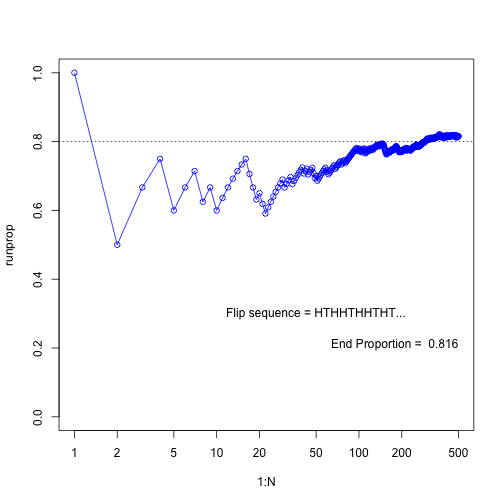
For the sample function in R one can give a vector of probabilities to the argument prob of the same length as the vector to sample from. Here, this allows to specify with which probability 0 or 1 are sampled.
Integral of Density
Normal density
mean <- 0
sd <- 0.2
xlow <- mean - 3*sd
xhigh <- mean + 3*sd
dx <- 0.02
x <- seq(xlow, xhigh, by=dx)
y <- 1/(sd*sqrt(2*pi))*exp(-1/2*(x-mean)^2/sd^2)
plot(x, y, type="h", lwd=1, ylab="p(x)")
lines(x, y)
# approximate integral
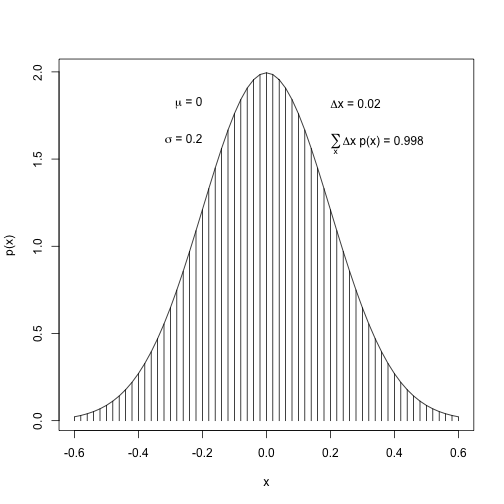
( area <- sum(y*dx) )
## [1] 0.9977213# add text to plot
# using function bquote
text(-sd, .9*max(y), adj=c(1,0),
labels=bquote( paste(mu, " = ", .(mean)) )
)
text(-sd, .8*max(y), adj=c(1,0),
labels=bquote( paste(sigma, " = ", .(sd)) )
)
text(sd, .9*max(y), adj=c(0,0),
labels=bquote( paste(Delta, "x = ", .(dx)) )
)
text(sd, .8*max(y), adj=c(0,0.5),
labels=bquote( paste(sum(,x,), Delta, "x p(x) = ", .(round(area, 3))) )
)
plot of chunk unnamed-chunk-8
#dev.copy2pdf(file="/Users/Claudius/Dropbox/Kruschke_Dog_Book/IntegralOfDensity.pdf")A new prob density function \(6x(1-x)\) defined over the range [0, 1]
Plot probability density function.
xlow = 0
xhigh = 1
dx = 1/1000
x = seq(from=0, to=1, by=dx)
y = 6*x*(1-x)
plot(x, y, type="l", xlab="x", ylab="prob. density")
lines(x, y, type="h", col="grey")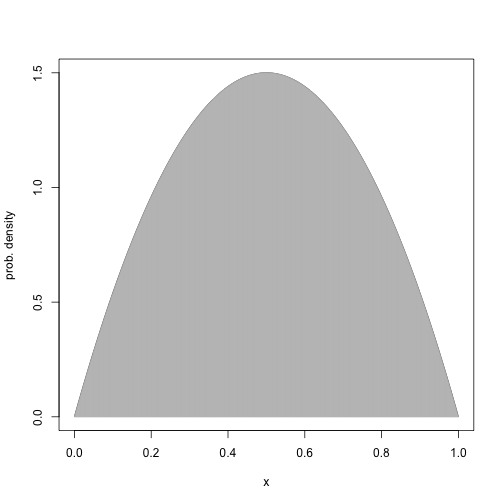
plot of chunk unnamed-chunk-9
Approximate the integral of the function over the range [0, 1].
approx_integral = sum( dx * y )
round(approx_integral, 2)
## [1] 1Get the mean and standard deviation of the function.
The mean can be calculated as in equation 4.7. It can also be approximated by splitting the continuous distribution of x into many intervals (as done above) and then using the probability that x falls into an interval as a weight for each x. This is done in the following:
# prob. density 'y' needs to be converted to a probability by multiplying it
# with the interval width
mu = sum( y*dx * x ) # see equation 4.5
mu
## [1] 0.4999995The same principal can be used to approximate the variance of this distribution:
\[ \begin{align} var(x) &= \int_{0}^{1} dx \quad p(x) [x-\mu]^{2} \\[5pt] var(x) &= \int_{0}^{1} dx \quad 6x(1-x)[x-0.5]^{2} \\[5pt] &= 0.05 \end{align} \]
var_x = sum( y*dx * (x-mu)^2 )
var_x
## [1] 0.04999975Now, let’s annotate the graph of the probability density with the values of its mean and standard deviation:
plot(x, y, type="l", xlab="x", ylab="prob. density")

label = bquote( paste( mu, " = ", .(round(mu, 1)) ) )
text(0, 1.4, label, pos=4)
label = bquote( paste( sigma, " = ", .(round(sqrt(var_x), 2)) ) )
text(0.8, 1.4, label, pos=4)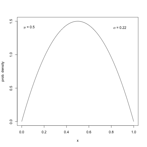
plot of chunk unnamed-chunk-13
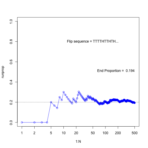
Exercise 3.1
N <- 500
flipseq <- sample(x=c(0,1), prob=c(0.8, 0.2), size=N, replace=T)
r <- cumsum(flipseq)
runprop <- r/(1:N)
plot(1:N, runprop, type="o", log="x", ylim=c(0,1), col="blue")
abline(a=0.2, b=0, lty=3)
flipletters <- paste( c("T", "H")[flipseq[1:10] +1], collapse="")
displaystring <- paste("Flip sequence = ", flipletters, "...", sep="")
text(50, 0.8, labels=displaystring)
text(N, 0.5, # coordinates
     paste("End Proportion = ", runprop[N]), # text
     adj=c(1,0) # right aligned
     )
plot of chunk unnamed-chunk-14
Exercise 3.3
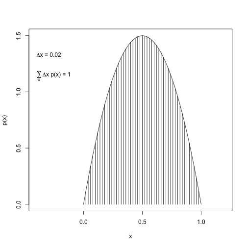
(A)
dx <- 0.02
x <- seq(from=0, to=1, by=dx)
y <- 6*x*(1-x)
plot(x, y, type="h", ylab="p(x)", xlim=c(-.4, 1.2))
lines(x,y)
( area <- sum(dx * y) )
## [1] 0.9996# add text to plot
text(-.4, .9*max(y), adj=c(0,1),
labels=bquote(paste(Delta, "x = ", .(dx)))
)
text(-.4, .8*max(y), adj=c(0,1),
labels=bquote( paste(sum(,x,), Delta, "x p(x) = ", .(round(area,3))) )
)
plot of chunk unnamed-chunk-15
(B)
\[ \begin{align} & \int_{0}^{1} 6x(1-x) dx \\[5pt] &= 6 \int_{0}^{1} x(1-x) dx \\[5pt] &= 6 \int_{0}^{1} x-x^2 dx \\[5pt] &= 6\left[\frac{1}{2}x^{2} - \frac{1}{3}x^{3}\right]_{0}^{1} \\[5pt] &= 6\left[\frac{1}{2} - \frac{1}{3} \right] \\[5pt] &= \frac{6}{2} - \frac{6}{3} \\[5pt] &= 3 - 2 \\[5pt] &= 1 \end{align} \]
Exercise 4.5
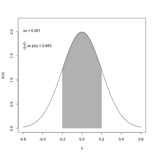
(A) Probability under normal curve between \(\mu-\sigma\) and \(\mu+\sigma\)
mean <- 0
sd <- 0.2
xlow <- mean - 3*sd
xhigh <- mean + 3*sd
dx <- 1/1000
x <- seq(from=xlow, to=xhigh, by=dx)
y <- 1/(sd*sqrt(2*pi))*exp(-1/2*(x-mean)^2/sd^2)
index <- (x >= -sd) & (x <= sd)
plot(x[index], y[index],
     type="h", col="grey",
     ylab="p(x)",
     xlab="x",
     xlim=c(mean-3*sd, mean+3*sd),
     ylim=c(0, 1.1*max(y))
     )
lines(x,y)
# approx. area by grid
( area <- sum(y[index] * dx) )
## [1] 0.6826885# exact area
( pnorm(sd, mean=0, sd=sd) - pnorm(-sd, mean=0, sd=sd) )## [1] 0.6826895# add text to plot
text(-.6, 2, adj=c(0,0),
labels=bquote(paste(Delta, "x = ", .(dx)))
)
text(-.6, 1.8, adj=c(0,1),
labels=bquote(
paste(
sum(, x=-sigma, x=sigma),
Delta, "x p(x) = ",
.(round(area,3))
)
)
)
plot of chunk unnamed-chunk-16
In a normal distribution, about 68% of the probability mass lies within one standard deviation around the mean.
(B)
mean <- 162
sd <- 177 - 162
curve(dnorm(x, mean, sd), from=162-3*sd, to=162+3*sd, ylab="p(x)")
abline(v=c(147, 177), lty=3)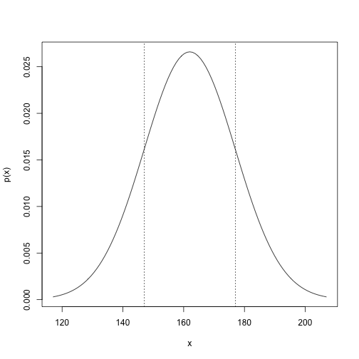
plot of chunk unnamed-chunk-17
Exercise 4.6
Food preferences among school children of different ages
# get the conditional probs into a matrix
cond.prob <- matrix(c(0.3,.6,.3,.6,.3,.1,.1,.1,.6),
              nrow=3, ncol=3,
               dimnames=list(c("1st graders", "2nd graders", "3rd graders"), c("Ice Cream", "Fruit", "French Fries")))
cond.prob
## Ice Cream Fruit French Fries
## 1st graders 0.3 0.6 0.1
## 2nd graders 0.6 0.3 0.1
## 3rd graders 0.3 0.1 0.6# get grade probs
grade.prob <- c(.2, .2, .6)
# multiply conditional prob by grade prob
# to get the conjoint prob of grade and food
( conjoint.prob <- cond.prob * grade.prob )## Ice Cream Fruit French Fries
## 1st graders 0.06 0.12 0.02
## 2nd graders 0.12 0.06 0.02
## 3rd graders 0.18 0.06 0.36If grade and food were independent, then the conjoint probabilities would be the same as the product of the two marginal probabilities for food and grade.
# marginal probabilities of the food
( marg.food <- colSums(conjoint.prob) )
## Ice Cream Fruit French Fries
## 0.36 0.24 0.40# marginal probabilities of the grade
# must be the same as grade.prob
( marg.grade <- rowSums(conjoint.prob) )## 1st graders 2nd graders 3rd graders
## 0.2 0.2 0.6conjoint.prob## Ice Cream Fruit French Fries
## 1st graders 0.06 0.12 0.02
## 2nd graders 0.12 0.06 0.02
## 3rd graders 0.18 0.06 0.36# get cross product of marginal probabilities
( indep.joint.prob <- outer(marg.grade, marg.food) )## Ice Cream Fruit French Fries
## 1st graders 0.072 0.048 0.08
## 2nd graders 0.072 0.048 0.08
## 3rd graders 0.216 0.144 0.24#class(marg.grade)
#class(t(as.vector(marg.food)))
#( indep.joint.prob <- as.vector(marg.grade) %*% t(as.vector(marg.food)) )
# get the difference between the joint probs. assuming independence of
# grade and food preference and the observed joint probs
( indep.joint.prob - conjoint.prob )## Ice Cream Fruit French Fries
## 1st graders 0.012 -0.072 0.06
## 2nd graders -0.048 -0.012 0.06
## 3rd graders 0.036 0.084 -0.12The table of conjoint probabilities cannot be reconstructed by multiplying grade and food probabilities, hence food and grade are not independent.
